双调排序(Bitonic Sort)
中文 | EN
为什么要用双调排序?
市面上已经有不少其他的排序算法,例如快速排序(quick sort)、蒂姆排序(Timsort)、堆排序(heap sort)、归并排序(merge sort)、希尔排序(shell sort)、冒泡排序(bubble sort)、选择排序(selection sort)和插入排序(insertion sort)等。
然而,上面作为例子的这些排序算法,无法在内存的确定位置处做比较,或者在确定位置处做元素交换。比如快排,它需要通过一个“支点(哨兵)”元素的值,将数组中的元素分为大于等于它和小于等于它的两部分。这个“支点”元素将成为一个“分水岭”,而“分水岭”的位置是不确定的。其他几种排序算法也有各自的不确定性。这意味着,要用GPU(特指GPGPU,亦即能做通用计算的GPU)来把它们变成并行算法的话,会遇到困难。
双调排序(bitonic sort)则解决了这个问题,所以它能方便地通过GPU来加速。它的发明人是Ken Batcher。
附记:“Batcher定理”是“Batcher排序”算法的理论基础。该算法是在双调排序算法之前被发明的。双调排序并不依赖于Batcher定理。当我写这篇文章(2022年9月)时,网上有很多文章在谈到双调排序的正确性证明时,说是用Batcher定理来证明。这是不对的。参见参考资料[1]。本文中,我将试图证明双调排序的正确性。
“双调”指的是什么?
它指的是一个非空的可排序序列(例如一个非空的整型数组)所显现的一种特性。这种特性是,这个序列要么是先递增后递减的,要么是先递减后递增的。注意,该特性也蕴含了以下几种特例:只递增、只递减、所有的值都是相等的。
双调排序是怎么做的
(声明:图片来自英文版维基百科)
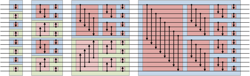
- 该算法从图的左边运行到右边。
- 图中的每个箭头代表一个“比较器”。箭头入口处的数组元素(比如一个数)被拿来与箭头出口处的数组元素比较,然后,当入口处的元素比较大时,它和出口处的元素将被对换位置。
- 每个蓝色或绿色盒子都从左边接受一个先上后下序列。这个序列是一半上升一半下降的,换句话说,上升部分的长度等于下降部分的长度。
- 蓝盒的输出是个递增序列。绿盒的输出是个递减序列。
来看一下红色盒子。如果把红色盒子竖着的一列看作一“层”,那么从左到右有多层红色盒子。红色盒子有一个长度,如2、4或者8。
- 如果某个红色盒子的长度是2,假设它的外面一层是蓝色盒子,那么该红色盒子会把较小的数放在左半边(数组中的左半边,或者是图中的上半边),把较大的数放在右半边。如果外面一层是绿色盒子,那么它把较小的数放在右边,较大的数放在左边。
- 如果某个红色盒子的长度是4,那么它的输出将带有以下特性:
- 特性1:假设外面一层是蓝色盒子的话,前一半的数小于等于后一半的数。
- 特性2:如果该红色盒子是外层蓝色盒子中的第一个红色盒子(也是这一层唯一的一个红色盒子),那么,输出的两半分别都是双调的。前一半是先增后减,后一半是先减后增。然而,前一半的先增后减并不保证是对半开的。后一半类似。(后面有详细解释)
- 特性3:在同一个蓝色盒子中,第二层或更后面层的红色盒子的输入并不能保证是对半开双调的。但这种输入是由前面一层的红色盒子产生的,所以带有它自己的“调性”。这一“调性”确保了它能被当前层的红色盒子正确地处理,并产生前一半的数小于等于后一半的数的效果。(后面有详细解释)
- 把所有这些特性综合起来,就能保证蓝色盒子的输出是递增的。
特性2的详解
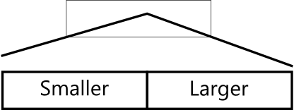
注:请对照前述的特性1和特性2来理解这些图。图中Smaller表示“更小些”,Larger表示“更大些”,意思是在输出中,左边一半的数小于等于右边一半的数。
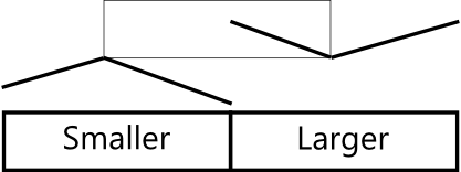
特性3的详解
注:请参考前述的特性3。当前一层的输出传给后一层时,有几种情况:
- 情况1:一半递增,一半递减的双调序列。这种情况比较容易理解,和蓝色盒子里第一个红色盒子遇到的情况类似。
- 情况2:先增后减的双调序列,但并非对半开。
- 情况3:由情况2的输入,经过红色盒子处理后,成为新的输出。参见后面的几张图。
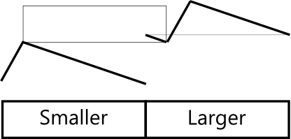
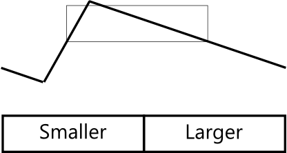
上面的几张图表示情况2。
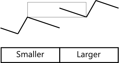
上面的几张图表示从情况2的右半边变成的情况3。
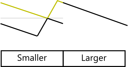
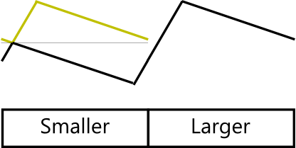
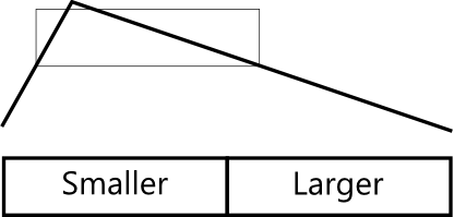
上面的几张图表示从情况3的两个半边分别变成的进一步的情况3。请着重看左半,黄绿色的线代表右半将有的输出。
可见,前一步输出的调性保证了后一步的输入最多不超过三种“调”。如果把左右两半都叠在左半,那么呈现出的是像“鱼”一样的形状。“鱼”的身子总是鼓的,鱼只有至多一个交叉点,而且“鱼身”的边界线也不会越过水平分界线(除了交叉点外)。这个就算不是完整的证明,也已经离完整的证明不远了。
历史上有一个完整的证明,用的是0-1原理。该原理及证明在1990年出版的《算法导论》第一版的第28章有详细讲解:[2]。
时空复杂度
我们讨论的是单线程的双调排序。它的时间复杂度很容易计算:每一层红色盒子需要O(n),总共有Log(n) ^ 2层,所以时间复杂度是O(n * Log(n) ^ 2)。
没有必要使用递归。也不需要动态分配空间。所以,空间复杂度是O(1)。
双调排序的Python程序
作者:范德成
运行示例
- Sequence: 5,9,2,8,4,3,7,1
- i: 0
- j, subStep, direction: 0, 2, 0
- i: 2
- j, subStep, direction: 0, 2, 1
- i: 4
- j, subStep, direction: 0, 2, 0
- i: 6
- j, subStep, direction: 0, 2, 1
- S: [5, 9, 8, 2, 3, 4, 7, 1]
- i: 0
- j, subStep, direction: 0, 4, 0
- j, subStep, direction: 1, 4, 0
- i: 4
- j, subStep, direction: 0, 4, 1
- j, subStep, direction: 1, 4, 1
- S: [5, 2, 8, 9, 7, 4, 3, 1]
- i: 0
- j, subStep, direction: 0, 2, 0
- i: 2
- j, subStep, direction: 0, 2, 0
- i: 4
- j, subStep, direction: 0, 2, 1
- i: 6
- j, subStep, direction: 0, 2, 1
- S: [2, 5, 8, 9, 7, 4, 3, 1]
- i: 0
- j, subStep, direction: 0, 8, 0
- j, subStep, direction: 1, 8, 0
- j, subStep, direction: 2, 8, 0
- j, subStep, direction: 3, 8, 0
- S: [2, 4, 3, 1, 7, 5, 8, 9]
- i: 0
- j, subStep, direction: 0, 4, 0
- j, subStep, direction: 1, 4, 0
- i: 4
- j, subStep, direction: 0, 4, 0
- j, subStep, direction: 1, 4, 0
- S: [2, 1, 3, 4, 7, 5, 8, 9]
- i: 0
- j, subStep, direction: 0, 2, 0
- i: 2
- j, subStep, direction: 0, 2, 0
- i: 4
- j, subStep, direction: 0, 2, 0
- i: 6
- j, subStep, direction: 0, 2, 0
- S: [1, 2, 3, 4, 5, 7, 8, 9]
- Sorted sequence: 1,2,3,4,5,7,8,9
怎么在GPU上实现一个双调排序呢?
GPU编程需要更多技巧。目前我还没实现出GPU上的双调排序。我试了以下简单的矩阵与向量相乘的程序。
简单地说,它需要pyopencl和numpy这两个库。Pyopencl是与OpenCL(Open Computing Language)集成的库。OpenCL实现了一种在GPGPU上运行的类C语言,并当GPGPU不存在时,回退到用CPU执行的模式。
有时间再来实现一个GPU上的双调排序。
参考资料:
中文 | EN
Why Bitonic Sort?
There are quite some well-known sorting algorithms available, such as quick sort, Timsort, heap sort, merge sort, shell sort, bubble sort, selection sort and insertion sort.
However, all the aforementioned sorting algorithms don't perform comparisons at pre-determined locations in memory, or swap items at pre-determined locations. For example, quick sort. It uses the value of a pivot item to divide the items in the array into two parts, one greater than or equal to it, and the other less than or equal to it. The pivot item will become a "dividing item". However, the location of the "dividing item" cannot be pre-determined. The other sorting algorithms have their location non-determinism as well. This hinders us when we want to parallelize them on a GPU (a General-Purpose GPU, or GPGPU, specifically).
Bitonic Sort solves this issue, and thus can be accelerated with a GPU. Its inventor is Ken Batcher.
Side note: The "Batcher Theorem" is the theoretic basis of "Batcher Sort". Batcher Sort was invented before Bitonic Sort was invented. Bitonic Sort doesn't rely on the "Batcher Theorem". When I am writing this article (September 2022), many articles on the Web talking about correctness of Bitonic Sort says that it can be proven with the Batcher Theorem. This is incorrect. See reference [1] for details. In this article, I will try to prove the correctness of Bitonic Sort.
What is bitonicity?
It is a property of a non-empty sortable sequence (such as a non-empty integer array). The property is that, the sequence is either ascending first, descending next, or descending first, ascending next. The property also implies three special cases: only ascending, only descending, all values are equal.
How the algorithm works
(Credit: Image is from Wikipedia.)
- The algorithm runs from the left to the right.
- Each arrow represents a comparator. The item (such as a number) at the start of the arrow is compared with the item at the end of the arrow, and they are swapped if the one at the start is greater.
- A blue or green box accepts from the left side an up-then-down bitonic sequence that is half-up and half-down. In other words, the up part has the same length as the down part.
- The output of a blue box is an ascending sequence. The output of a green box is a descending sequence.
Consider the red boxes. If we view a column of red boxes as a "layer", then there are multiple layers of red boxes from the left to the right. A red box has a length, which is like 2, 4 or 8.
- If the red box length is 2, suppose the box surrounding it is a blue box, essentially the red box puts smaller numbers in the left half (the left half of an array, or the upper half seen on the diagram) and larger numbers in the right half. Or the smaller on the right and the bigger on the left if the outer box is green.
- If the red box length is 4 or more, it will achieve the following properties in the output:
- *PROPERTY1* The first half numbers are less than or equal to those in the second half, if the outer box is blue.
- *PROPERTY2* If the red box is the first one in the outer blue box (which is also the only red box in the layer), the two halves of the output sequence are both bitonic. The first half is up-then-down. The second half is down-then-up. However, the first half isn't guaranteed to be half-half bitonic. Same for the second half. (Explanations will follow.)
- *PROPERTY3* In the same blue box, input to a red box in the second or a later layer isn't guaranteed to be half-half bitonic. However, the input is generated by a red box of the previous layer, so it has its own bitonicity. This bitonicity guarantees that it will be processed properly by the current red box in the current layer, and generates a half-smaller half-larger output. (Explanations will follow.)
- These properties together guarantee that the output sequence of a blue box is ascending.
Explanations of PROPERTY2
Note: please try to understand these diagrams according to PROPERTY1 and PROPERTY2 mentioned earlier.
Explanations of PROPERTY3
Note: please try to understand these diagrams according to PROPERTY3 mentioned earlier. When the output from the one layer is passed to the next layer, there are several different cases:
- Case 1: half up and half down bitonic. This is trivial. It is similar to the situation of the first red box in a blue box.
- Case 2: up and down bitonic, but not half up and half down.
- Case 3: the input of this case is the output of case 2.
The diagrams above show the case 2.
The diagrams above show how the right half of case 2 becomes the case 3.
The diagrams above show how the two halves of case 3 becomes two new case 3 outputs. Look at the left half, where the greenish-yellowish line represents the right half of the output.
As you have seen, the tonicity of the input guarantees that there are at most three tones in the output. If you double the right half on the left half, the shape is like a "fish". The body of the fish is always "bulging". There is at most one converge point. And the body lines of the fish never cross the horizontal dividing line, except for the converge point. It is nearly a complete proof, if not a complete proof.
In history, there is a complete proof based on the 0-1 principle. The principle and the proof are described in detail in Chapter 28 of the book Introduction to Algorithms, first edition: [2]。
Time and space complexity
When we say time complexity, we always mean the single-threaded case. The time complexity is quite apparent: Each red box level needs O(n), and there are Log(n) ^ 2 levels, so it's O(n * Log(n) ^ 2).
There is no need to use recursion. No dynamic memory allocation is needed. So, the space complexity is O(1).
A python implementation of bitonic sort
Author: Decheng Fan
A sample run
- Sequence: 5,9,2,8,4,3,7,1
- i: 0
- j, subStep, direction: 0, 2, 0
- i: 2
- j, subStep, direction: 0, 2, 1
- i: 4
- j, subStep, direction: 0, 2, 0
- i: 6
- j, subStep, direction: 0, 2, 1
- S: [5, 9, 8, 2, 3, 4, 7, 1]
- i: 0
- j, subStep, direction: 0, 4, 0
- j, subStep, direction: 1, 4, 0
- i: 4
- j, subStep, direction: 0, 4, 1
- j, subStep, direction: 1, 4, 1
- S: [5, 2, 8, 9, 7, 4, 3, 1]
- i: 0
- j, subStep, direction: 0, 2, 0
- i: 2
- j, subStep, direction: 0, 2, 0
- i: 4
- j, subStep, direction: 0, 2, 1
- i: 6
- j, subStep, direction: 0, 2, 1
- S: [2, 5, 8, 9, 7, 4, 3, 1]
- i: 0
- j, subStep, direction: 0, 8, 0
- j, subStep, direction: 1, 8, 0
- j, subStep, direction: 2, 8, 0
- j, subStep, direction: 3, 8, 0
- S: [2, 4, 3, 1, 7, 5, 8, 9]
- i: 0
- j, subStep, direction: 0, 4, 0
- j, subStep, direction: 1, 4, 0
- i: 4
- j, subStep, direction: 0, 4, 0
- j, subStep, direction: 1, 4, 0
- S: [2, 1, 3, 4, 7, 5, 8, 9]
- i: 0
- j, subStep, direction: 0, 2, 0
- i: 2
- j, subStep, direction: 0, 2, 0
- i: 4
- j, subStep, direction: 0, 2, 0
- i: 6
- j, subStep, direction: 0, 2, 0
- S: [1, 2, 3, 4, 5, 7, 8, 9]
- Sorted sequence: 1,2,3,4,5,7,8,9
What about GPU?
GPU programming requires more technique. I haven't implemented bitonic sort on GPU yet. I tried out simple matrix-vector multiplication.
Basically, it requires pyopencl and numpy libraries. Pyopencl is a library that integrates with OpenCL (Open Computing Language), which implements a C-like language that runs on GPGPU (and falls back to CPU if there is no GPGPU).
When time allows, I will implement a fast bitonic sort on GPU.
References:
[2] Sorting Networks - Chapter 28 of Introduction to Algorithms, first edition